METHODS FOR MULTIPLE DESCRIPTION (MD) CODING
There are several different techniques for multiple description coding but basically one can categorize them into three different approaches:
· Quantization based
· Transformation based
· Mixed transformation/quantization based
Herein, we try to give a brief introduction
to some of the methods used. For detailed descriptions on the different
techniques and rate-distortion analysis
please resort to the material in the reference list.
MD Quantization
A quantizer can be divided into an encoder
part and a decoder part. The encoder takes the source sample (vector), which is
real valued, and maps
it to a codeword index. Since this is a many-to-one mapping we will generally
never be able to reconstruct the source sample exactly.
The decoder maps the codeword index from the encoder to a reconstruction source sample vector.
Encoder ![]() :
: ![]()
Decoder ![]() :
: ![]()
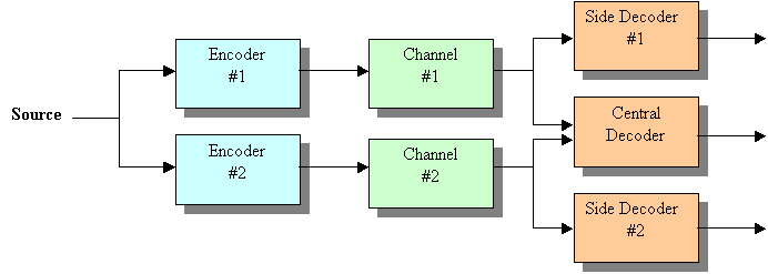
Multiple description quantizers can conceptually
be seen as the use of a set of independent scalar (or vector) quantizers to
obtain
a number of descriptions of a source sample (vector). Each description is then
transmitted (in packets) to the receiver using as many channels as
descriptions.
The channel is assumed to only introduce packet loss errors.
At the receiver the source sample (vector) is reconstructed by combining the descriptions arrived. The more descriptions that arrive at the receiver the lower the distortion between the original and reconstructed source sample (vector) becomes. Note that if we would transmit the same description over all channels we would only gain in terms of reducing the probability of a description not to arrive at the receiver, but we could never reduce the quantization error by receiving more than one description.
The figure below depicts an MD quantization scheme having two quantizers.
Reconstructed Source

MD Scalar Quantization (MDSQ)
The simplest scenario is to have two scalar quantizers with nested cell
borders:
Q1
![]()
Q2
![]()
Q0
![]()
Q2
It is obvious now that in this example the central decoder (D0) has about 4 times less distortion compared to the distortion for the side decoders (D1,,D2) since the intersection cells are half as big as for the side decoders.
The simple example above is just one out of infinite number of ways on how to design a MDSQ.
What is commonly done is that one tries to minimize the average distortion of the central decoder under constraints on the distortions for the side decoders.
The Lagrangian optimization then basically becomes the known Lloyd iterations:
- Find the optimal decoder given the encoder
- Find the optimal encoder (partitioning) given the decoder
Not just how the cell boundaries are placed determines the performance but also the index assignment.
See for instance [Vaishampayan, 1993] for detailed design strategies and rate-distortion bounds for MDSQ.
Just as it is possible to construct vector quantizers (VQ) that outperform scalar quantizers it is possible to have multiple description vector quantizers, MDVQ, that improve upon the performance of MDSQ. The underlying principle for MDVQ and MDSQ is the same [Kelner et al., 2000].
MD Transform Coding
MDTC based on Statistical redundancy
The main idea of MDTC based on statistical redundancy is to transform the source signal twice. The first transform decorrelates the source and the second transform reintroduces correlation but in a controlled manner.
Orthogonal MDTC:
The orthogonal (orthonormal) MDTC is
basically a rotation of the basis functions onto which the source sample vector
is projected to introduce dependency between the original uncorrelated
(independent in the Gaussian case) source samples. After the rotation is
performed scalar quantizers are applied and the resulting indices are entropy
coded and transmitted over the channels to the decoder (see figure below).
Source

A great advantage by applying the orthogonal transform (rotation) is that we are able to reduce the distortion at the side decoder when we have lost one description. This is possible since we by the introduction of statistical dependencies between the variables are able to obtain a prediction of the lost variable based on the received one.
Consider for example the simple case with
an orthonormal transform that rotates the source sample vector ![]() by 45 degrees
by 45 degrees
 ,
,
where we in this example assume that the source sample vector ![]() is jointly Gaussian with
a diagonal covariance matrix
is jointly Gaussian with
a diagonal covariance matrix  .
.
If we neglect the quantization and assume
that the packet containing ![]() gets lost we can still obtain estimates of the original
source sample vector by replacing
gets lost we can still obtain estimates of the original
source sample vector by replacing ![]() by
by ![]() and applying the
inverse transform, i.e.,
and applying the
inverse transform, i.e.,
 .
.
Furthermore, it can be shown that ![]() is Gaussian with mean
is Gaussian with mean
 .
.
Everything has its price and here the price is that we by decreasing the side distortions we are increasing the central distortion.
Using different orthonormal transforms one can have different trade-offs between side and central distortions.
Nonorthogonal MDTC:
Having a nonorthogonal transform instead of an orthogonal transform gives an increased variability for different trade-offs between the side and central distortions.
A problem is that uniform scalar quantizers on nonorthogonal transformed variables results in nonhypercubic partition cells, which are suboptimal for scalar quantizers. However, this can be overcome by placing the scalar quantizer before the transform. The continuous transform has now to be replaced by a discrete integer-to-integer transform.


Goyal and Kovacevic introduce the following integer-to-integer transform (for the case of two source samples in a vector) [Goyal et al., 1998a] [Goyal et al., 2001a] [Kovacevic et al., 1998]:
![]()
with det( T ) = 1. The transform can be factored as
 .
.
The discrete transform then becomes
![]() ,
,
where ![]() represents quantization to the nearest multiple of the
quantization step-size
represents quantization to the nearest multiple of the
quantization step-size ![]() .
.
The inverse transform becomes
![]() .
.
If some components of ![]() are lost, they are estimated from the received components by
means of the statistical correlation introduced by
are lost, they are estimated from the received components by
means of the statistical correlation introduced by ![]() (like in the simple
example on the reconstruction from the orthogonal transform).
(like in the simple
example on the reconstruction from the orthogonal transform).
Optimal design procedure [Goyal et al., 1998a] [Goyal et al., 2001a]:
·
Choose a weighted average distortion ![]() .
.
· Choose a target rate R.
· Numerical minimization gives T.
· Use discrete version of T.
MDTC based on Frame theory
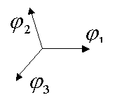
A frame is a set of nonindependent vectors,![]() , that satisfies the following condition
, that satisfies the following condition
![]() ,
,
where ![]() and
and ![]() for all
for all ![]() . The frame is said to be tight if the frame bounds are
equal,
. The frame is said to be tight if the frame bounds are
equal,![]() . For a tight frame the frame bound gives the redundancy
ratio. If the redundancy ratio is equal to 1, then the frame is just an
orthonormal basis and, thus, the tight frame can be seen as a generalization of
orthonormal bases to having more vectors than a basis.
. For a tight frame the frame bound gives the redundancy
ratio. If the redundancy ratio is equal to 1, then the frame is just an
orthonormal basis and, thus, the tight frame can be seen as a generalization of
orthonormal bases to having more vectors than a basis.
Example of a tight frame with a redundancy ratio of 1.5 (since we use 3 vectors describing the 2D space) can be seen below.

The frame expansion function is simply the
inner product between the vector of source samples and the set of frame
vectors, i.e.,![]() .
.
For tight frames the dual frame (inverse
operator) is the frame itself normalized with the frame bound, i.e., ![]() .
.
The idea is then to from the original source sample vector of dimension N use the frame expansion to have a new vector of dimension M (M>N) with dependent elements and then apply a scalar quantizer before transmission. The scheme is depicted in the figure below.

If we receive all samples then applying the
dual frame does the reconstruction of the source sample vector. Otherwise if
the number of erasures is ![]() , the dual frame without the columns corresponding to the
missing samples is used for the reconstruction. For more than M - N
errors the reconstruction is impossible.
, the dual frame without the columns corresponding to the
missing samples is used for the reconstruction. For more than M - N
errors the reconstruction is impossible.

For details on how to construct tight frames and performance evaluations see for instance references [Kovacevic et al., 1998], [Goyal et al., 1998b], [Goyal et al., 2001b].